
The introvert’s guide to visiting every country
Published:
Hey everyone! Gather around, another one of my random thought experiment + vibe coding + optimization + plotting blogs is here!
The idea for this started many months ago when I was playing around with the map from Patrick Stolz. I wrote about it previously here where I visualized all the places I’ve visited so far and calculated a “Travel Score.” What fascinated me about the original dataset was this beautiful mapping: Population distribution ⇔ Geographic coordinates ⇔ Countries. I mean, come on, if that doesn’t scream “turn me into an optimization problem,” are you even a nerd?
Anyway, the idea that popped into my head was this: what if I were an introvert (I’m not) who still wanted to travel the world (which I do)? And I wanted to visit all 197 countries (as listed in the dataset) while meeting the least possible number of people. Now that’s a fun project I can get behind!
With that idea, it was time to sit down with the data and preprocess it into an easier format. The original data had a much more complicated structure than I liked. The first thing I did was to write the data in a way my simple human brain could understand — a CSV file with grid ID, percentage of population, percentage of land area covered by this grid, and the list of countries this grid maps to. I vibe-coded this from all the complicated files in the original dataset. This one file should be sufficient to start with the optimization algorithm, but as you will see soon, I needed a second file — one where I could connect the grid ID to the geographical coordinates (think of a polygon with each vertex given by its latitude and longitude). These are the grids we see in the original map. This second mapping would come in handy for extending the optimization to a more “realistic” scenario.
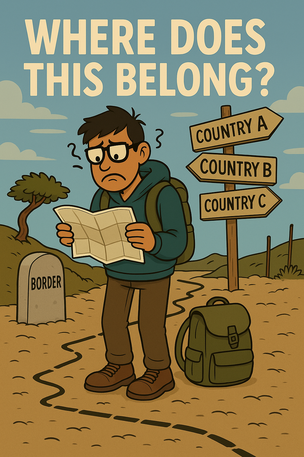
After I started thinking more about this, I realized this is not one optimization but can be expanded into multiple ones based on the assumptions I had made. Here are a few thoughts I can explain before jumping into the algorithms and results (which I know all of you are eager to find out! /s :D). So, the first thing to know is, each grid ID might map to more than one country. Second, for every grid ID we only know the percentage of the population of the world (according to some dataset in some unknown-to-me year), but we do not have country-wise distribution. Now, this introduces our first challenge — assuming we have an optimization algorithm and it picks a grid ID, do we assume we have visited all the countries that correspond to this grid ID or only one country? If only one country, how do we select which country?
As it often turns out, one assumption makes your algorithm trivially easy, and removing that assumption makes the algorithm wildly difficult. This turned out to be such an assumption. Let’s look at the two cases below.
Case 1: All Grids, All Countries Per Grid (Simple Greedy)
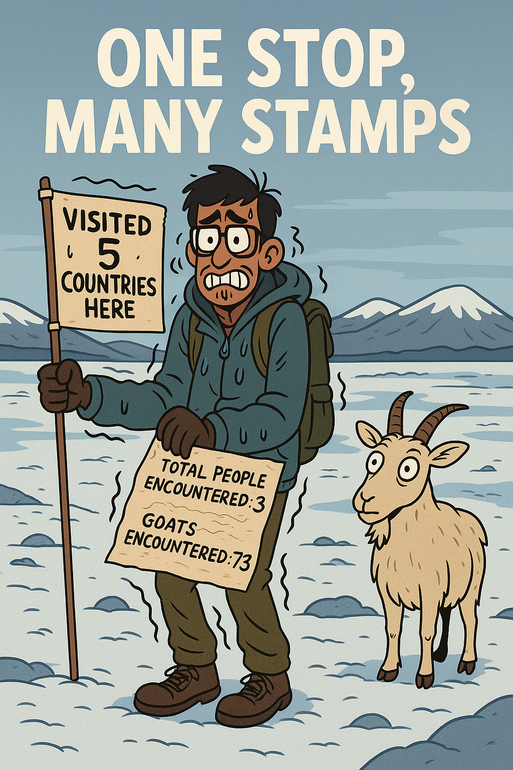
This is a baby in the world of optimization problems — I pick the lowest population grid per country. If a grid belongs to multiple countries — great! One stop, many stamps. Ok, this is pretty easy (even for me, let alone my Claude-4-powered Cursor) to implement. One prompt, booooom! Implemented, done, time for coffee now. (I did not verify that this is indeed the theoretical minimum though. You will see with the results that they seem reasonable to me.)
Case 2: All Grids, One Country Per Grid (Hungarian Algorithm)
Ok, this was a tough nut to crack. I don’t even know how to start — maybe Cursor does?

Wow, “THOUGHT FOR 15 seconds”!!! This one drove me down a rabbit hole — I ended up reading (and not really understanding) the assignment problem and apparently something called the Hungarian algorithm. (Turns out this algorithm was developed by Harold Kuhn, the person who represents the second 'K' in the famous KKT condition in optimization.) Had never heard of that before. These random pursuits do teach me some new concepts! Anyway, back to our problem — this turned out to be much harder to understand and also to get working with the vibe code. It’s still amazing to see how these LLMs can help in actual scientific computing. They can not only do text and simple boilerplate code but actual realistic scientific computing. The caveat, as always, is: if this were to be a real scientific research or engineering product, I would need to ENSURE that the produced code is correct. However, this is just my random curiosity code, so I can live with some tolerance for issues in the code. One thing I had to account for, though, is that there were a few cases (two cases to be exact) where there were two or more countries in exactly one single grid and nowhere else (think of two tiny island nations next to each other — they would share the grid ID and would only be in this one single grid ID. If I assign this grid ID to one, then I can never visit the other unless I reassign the same grid ID).
Now, this is where I started comparing the optimum values (which were in the range of 1–3% of the world population) with my own travel map. As of this writing, I have visited 46 countries, but my population encountered was a whopping 25%!!! Unrealistic as it might be that I have “met” 2 billion people, this got me wondering how it is that the algorithm chooses these amazing (for an introvert) locations. Then it hit me — of course, I fly to many of the places (I know, I am guilty of my CO2 emissions — I have written about it earlier here), and flying is often to big cities which would have high population percentages. (And of course, the fact that I am from India accounts for a lot of the “population encountered”!)
The previous optimization would pick grids and assume that an introvert traveller would just teleport between these grids somehow. That is, of course, unrealistic (at least more unrealistic than the premise of this blog), and as anyone already down this path would normally do, I went around looking for a dataset with all airports and landing strips in the world. And surprise, surprise — it exists and is easily available in a simple CSV file. Now the next logical step was to incorporate this into my optimization. This is where the second file I had mentioned before comes in. The airport data comes with the latitude and longitude of each airport. I reverse-mapped this to grid IDs — meaning, for each airport I mapped which grid it was in. To save this reverse mapping, I needed the polygonal data of each of the grids. Ok, now we fly!
Case 3: Airports, Shared Country Grids (Greedy + TSP)
The next case was to use only the grids which have airports as options for us to visit. We can reuse the greedy cover set as before. However, we still have the case that a selected grid (with an airport) could be associated with multiple countries. Now, this is like saying the traveller flew into a specific airport in one country and visited the nearby countries (that are in the same grid) by land, sea, zipline, burro, or whatever. This is quite realistic, of course. Running this algorithm was quite easy, but it quickly turned out that the airports chosen are super unknown — like Random-city-landing-strip-03. Anyway, I was able to pick the full set of airports. Now, given that this worked out, I thought why not throw in my CO2 calculation for such a trip? I had the code lying around, and with one prompt, Claude-4 just integrated it into my code here. I went one step further — after integrating the CO2 calculation between all selected airports to all other selected airports, I ran the TSP algorithm to optimize my route. Now I can travel the world, avoid people, and also feel slightly less guilty about flying in an unoptimized way. Again, the TSP was included just because I had the code lying around from yet another earlier blog project (I know! Shameless plug to my own previous blog!). To mitigate this random one-landing-strip-to-random-other-landing-strip flight, I would need to find more realistic commercial flight data and maybe use that. I can keep this for another day though. This version introduced “real-world” logistics and a CO2 tracker to account for emissions.

Case 4: Airports, Host Country Only (Hardcore Realism)
Finally, coming to the strictest and cleanest version, where you only strictly fly. You can only count a country if you fly into an airport grid hosted by that country — no border-hopping. This was a bit more challenging than I had anticipated, basically because some countries either do not have airports or the airport database does not assign them correctly. The code processes this first by assigning the airports to host countries. (A side challenge was to ensure that the names of countries in the airport database match the population dataset. I did this by mapping everything into ISO names with some extra mappings just for guarantees.) After assigning host countries, we process countries without airports by checking if there are other airports in the same grid but in a different country. If yes (and it is a yes in EVERY case we consider), we assign the same airport to both countries. Anyway, after this, we throw in the CO2 and the TSP as before. This is probably not as realistic as the previous case, but I thought it would be incomplete without this version. Finally, for fun, below is a CO2-emission-optimized travel map visiting every country in the world by flying. (Note: The dashed red lines represent crossing the date line and due to plotting limitations, they seem like we are zipping across the world in an "unoptimized" way.)

🌍 Introvert Travel Route
Results
Finally, what everyone (anyone?) has been waiting for!!! How do each of these algorithms stack up against each other? Well, my intuition said the first should be the best (or worst, depending on how you swing) in terms of people encountered, and the fourth being the worst. However, I was not sure of the ordering between 2 and 3. Turns out, limiting ourselves to airport-only grids is almost as good as the free-to-choose-any-grid option. This reinforces the idea that we have a lot of unheard of landing strips and airports in that dataset. Maybe I really need to find that flight connections data after all! The table below summarizes the percent of global population “met” during the journey for each case:
| Case | Travel Mode | Grid Constraint | Country Constraint | Population % Encountered |
|---|---|---|---|---|
| 1 | Teleport | Any | Shared countries OK | 1.15% |
| 2 | Teleport | Any | Unique per country | 1.58% |
| 3 | Flights | Airports only | Shared countries OK | 1.22% |
| 4 | Flights | Airports only | Unique per country (Host country) | 3.70% |
Looking at the table, it was an interesting exercise for me to learn that by flying into remote locations, one can visit all 197 countries and practically encounter <4% of the world (well obviously, we won’t meet everyone in that grid, but it is fair to assume that the number of people we encounter is proportional to the population percentage in that grid). For the people (aka weirdos) who want to play with the code, I will upload it on GitHub.
PS: I also wanted to try character consistency in the 4o model in just single step like the viral videos were showing. So the images were generated just for fun and to keep the blog more visually appealing.